:: Table of Contents

picture

LaTeX's picture environment draws diagrams from coordinates: lines, arrows, circles, curves and polygons, with text and maths placed wherever they are needed. fxTeX Pro draws each picture as SVG, inside the equation, so a labelled triangle, a vector or a pair of axes can sit in a sentence or beside an equation like any other piece of maths. The labels stay live: in the editor below, each one is typed in place, and an empty one is a box waiting to be filled. The picture panel holds ready-made shapes, and its first button opens the picture editor, to draw a picture of your own. Click any example on this page to open it there.

Compiling the same pictures in LaTeX? Everything on this page is standard LaTeX — the picture environment and pict2e's extras — with one small addition: dashed and dotted lines. Those come from fxpicture.sty, our package for LaTeX. Add \usepackage{fxpicture} to your preamble and every picture made here compiles in pdfLaTeX, LuaLaTeX or XeLaTeX, drawn the same as it is on this page. More about fxpicture.

Download fxpicture.zip

Adding picture to your page

In fxTeX Pro, name picture when you render the page:

fxTeXPro.ready.then(() => {
  fxTeXPro.unlock('fx_pk_your-key-here');
  fxTeXPro.autoRender({ packages: ['picture'] });
});

In the equation editor, name it to EqEditor.init() and add the picture panel to the toolbar. This is the editor above:

<script src="https://fxeditor.codecogs.com/fxeditor.api.min.js"></script>

<div id="toolbar"></div>
<div id="mathview"></div>
<div id="latex"></div>

<script>
  const ready = EqEditor.init({
    licence: 'fx_pk_your-key-here',
    packages: ['picture']
  });

  const toolbar = EqEditor.Toolbar.link('toolbar', [
    ['picture', 'geometry', 'operators_core', 'brackets', 'arrows'],
    ['greeklower', 'greekupper', 'relations', 'symbols', 'accents', 'spaces', 'colors']
  ]);

  ready.then(() => {
    const latex = EqEditor.LaTeXView.link('latex');
    const mathview = EqEditor.MathView.link('mathview').addLaTeXView(latex);
    toolbar.addLaTeXView(latex).addMathView(mathview);
    mathview.setLatex('\\begin{picture}(50,50)(-25,-25)\\put(0,0){\\circle{50}}\\end{picture}');
  });
</script>

The picture panel has triangles, quadrilaterals, circles, axes, grids and solids, each with its labels left empty to fill in, and a button that opens the picture editor on a new picture or on the one the caret is in. picture adds 77 kB gzipped: name it only on the pages that use it. See Using packages for more on both steps.

The picture editor

To draw a picture of your own, or change one, open the picture editor: press the first button of the picture panel, click a picture's lines in the equation, or double-click anywhere on it. A page can open it on its own with EqEditor.PictureEditor.open(latex), which resolves with the new LaTeX, or null if the reader cancels.

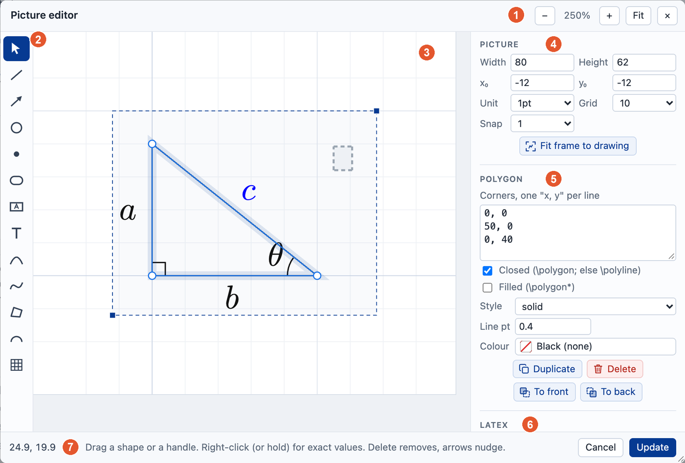
Zoom and close. Zoom out and in (or Ctrl+wheel), Fit to show the whole picture, and × to close without saving. Drag the title bar to move the dialog, and its corner to resize it.
Tools. Select, then line, arrow, circle, dot, oval, box, text, quadratic and cubic curves, polygon, arc and grid. Each has a key: hover over a tool to see it.
The drawing. Drag with a tool to draw, or click for a shape of a sensible size. Drag a shape to move it, or one of its handles to move that point; the arrow keys nudge. Points snap to the grid, and to other shapes' corners, so lines meet. Shift+click, or a box dragged round them, selects several shapes. Right-click a shape or a handle (press and hold, on a touch screen) to type its exact values. A dashed box is a label left empty, which the reader fills in later, in the equation.
Picture. The size of the picture and its lower-left corner, the unit its numbers are in, and the grid and snap. Fit frame to drawing sizes the picture to what is drawn.
Shape. Everything about the selected shape: its points, whether it is closed or filled, its line style, width and colour - and buttons to duplicate or delete it, and move it in front of or behind the others. A label has its text here, with a Maths box to set it in maths.
LaTeX. The picture as it will go into the equation. Edit it here and the drawing follows.
Status. The pointer's position, in the picture's units, and a hint for the tool in use. Update (or Insert, for a new picture) puts the picture into the equation; Cancel leaves it as it was.

Lines and arrows

\begin{picture}(w,h) sets the picture's size, and (x0,y0) after it, if given, its lower-left corner. \put(x,y){...} places anything at a point. \line(a,b){len} and \vector(a,b){len} take a slope and a length; pict2e's \Line(x1,y1)(x2,y2) joins two points.

\begin{picture}(60,40)\put(0,0){\line(1,0){60}}\put(0,0){\line(3,2){60}}\put(0,0){\vector(0,1){40}}\end{picture}

Lines and an arrow, from one point.

\begin{picture}(60,40)\Line(0,0)(60,40)\Line(0,40)(60,0)\end{picture}

\Line: from one point to another.

\begin{picture}(70,50)(-5,-5)\thicklines\put(0,0){\vector(1,0){60}}\put(0,0){\vector(0,1){40}}\thinlines\put(62,-2){$x$}\put(-2,42){$y$}\qbezier(0,0)(30,40)(60,0)\end{picture}

𝑥 𝑦

Axes, labelled, with a curve.

\begin{picture}(60,30)\multiput(0,0)(10,0){7}{\line(0,1){30}}\multiput(0,0)(0,10){4}{\line(1,0){60}}\end{picture}

\multiput: the same thing, again and again.

Circles, ovals and polygons

\circle{d} is a circle of diameter d, \circle* a filled one. \oval(w,h) has rounded corners, and [t], [bl] and the like draw only part of it. \arc[a1,a2]{r}, \polygon and \polyline are pict2e's.

\begin{picture}(50,50)(-25,-25)\put(0,0){\circle{50}}\put(0,0){\circle*{3}}\put(0,0){\line(1,0){25}}\put(10,2){$r$}\end{picture}

𝑟

A circle, its centre and its radius.

\begin{picture}(80,50)\put(40,25){\oval(70,40)}\put(40,25){\oval(40,20)[t]}\end{picture}

An oval, and the top half of another.

\begin{picture}(50,50)\polygon(0,0)(50,0)(25,43)\polygon*(20,10)(30,10)(25,19)\put(25,20){\arc[0,180]{15}}\end{picture}

A triangle, a filled one inside it, and an arc.

\begin{picture}(60,30)\polyline(0,0)(15,30)(30,0)(45,30)(60,0)\end{picture}

\polyline: a path through the points, left open.

Curves

\qbezier is a quadratic Bézier curve, through its first and last points and pulled towards the middle one; pict2e's \cbezier is a cubic one, with two. A number in square brackets draws the curve as that many dots.

\begin{picture}(80,40)\cbezier(0,0)(20,40)(60,-20)(80,20)\put(0,0){\circle*{2}}\put(80,20){\circle*{2}}\end{picture}

A cubic curve, its ends marked.

\begin{picture}(60,30)\qbezier[20](0,0)(30,40)(60,0)\end{picture}

A curve drawn as 20 dots.

Labels and boxes

What \put places is text, as in LaTeX: put maths in $...$ . \makebox, \framebox and \dashbox set text in a box of a given size; \color colours what follows it. A picture can sit inside an equation, on its baseline.

\begin{picture}(58,54)(-11,-12)\polygon(0,0)(45,0)(0,40)\polyline(4,0)(4,4)(0,4)\put(-9,17){$a$}\put(20,-10){$b$}\put(25,23){$c$}\end{picture}

𝑎 𝑏 𝑐

A right-angled triangle, its sides labelled.

x + \begin{picture}(40,20)\put(0,0){\framebox(40,20){box}}\end{picture} = y

x + b o x = y

A picture in an equation.

\begin{picture}(60,40)\put(0,0){\makebox(60,40)[tl]{TL}}\put(0,0){\makebox(60,40)[br]{BR}}\put(0,0){\dashbox{3}(60,40){$\frac{a}{b}$}}\end{picture}

T L B R 𝑎 𝑏

Text placed in a box's corners, and maths in a dashed box.

\begin{picture}(60,40)\color{red}\put(0,0){\line(1,1){40}}{\color{blue}\put(10,30){blue text}}\put(40,0){\circle{10}}\end{picture}

b l u e t e x t

Colour, kept to its group.

Dashed and dotted lines

The one thing here that is not in LaTeX already. \linestyle{dashed}, dotted or dashdot — or \dashpattern{on}{off}, a pattern of your own — applies to every line, curve and outline after it, to the end of its group, the way \linethickness does. \linestyle{solid} goes back to solid lines. To compile these in LaTeX, load fxpicture.

\begin{picture}(60,40){\linestyle{dashed}\put(10,10){\line(1,0){40}}\put(10,20){\oval(40,10)}\put(10,30){\qbezier(0,0)(20,15)(40,0)}}\end{picture}

Dashed: a line, an oval and a curve.

\begin{picture}(80,40)\linestyle{dotted}\put(0,35){\line(1,0){80}}\put(15,15){\circle{24}}\thicklines\linestyle{dashdot}\put(35,5){\vector(1,0){45}}\put(35,20){\vector(2,1){30}}\end{picture}

Dotted, then dash-dot arrows.

\begin{picture}(80,40)\dashpattern{3pt}{2pt}\polygon(0,0)(30,0)(15,25)\put(55,15){\arc[0,270]{12}}\linestyle{solid}\put(0,35){\line(1,0){80}}\end{picture}

A pattern of your own, then solid again.

Grids

\grid(w,h)(dx,dy) draws lines every dx across and every dy up; with [x0,y0] after it, each line is numbered, counting from there. It is epic's \grid, which fxpicture provides in LaTeX too.

\begin{picture}(60,40)\put(0,0){\grid(60,40)(10,10)}\put(9,27){\line(1,1){21}}\end{picture}

A grid to draw on.

\begin{picture}(60,40)\put(0,0){\grid(60,40)(10,10)[0,0]}\end{picture}

00101020203030404050506060001010202030304040

Numbered from 0.

Units and coordinates

A bare number is a multiple of \unitlength, 1pt unless it is set; a length with a unit is that length. Lengths can be added, subtracted, multiplied and divided.

\setlength{\unitlength}{1mm}\begin{picture}(30,20)\put(0,0){\line(3,2){30}}\put(15,10){\circle{5}}\end{picture}

Measured in millimetres.

\begin{picture}(2cm,1cm)\put(0,0){\line(1,0){2cm}}\put(1cm,0.5cm){\circle*{3pt}}\put(0.5cm+2pt,0){\line(0,1){1cm}}\end{picture}

Lengths with units, and a sum.

Not read, and drawn as nothing: \graphpaper, pict2e's path commands (\moveto, \lineto, \strokepath), \bezier, \savebox and \usebox.

fxpicture.sty: the same pictures in LaTeX

A picture made here is LaTeX, and compiles in a LaTeX document. Most of it needs nothing more than LaTeX itself and pict2e, which every current TeX distribution has. The exception is line styles: LaTeX draws every line solid, and has no way to dash one. fxpicture is our package that adds them — a small change on top of pict2e, and only that. It adds \linestyle and \dashpattern as an option; a picture that does not use them comes out exactly as pict2e draws it, and so does every solid line in one that does.

\documentclass{article}
\usepackage{fxpicture}   % loads pict2e, and passes any options on to it

\begin{document}
\begin{picture}(60,40)
  {\linestyle{dashed}
    \put(10,10){\line(1,0){40}}
    \put(10,20){\oval(40,10)}
  }
  \put(10,30){\line(1,0){40}}   % solid again, after the group
\end{picture}
\end{document}

Declaration	Draws lines
`\linestyle{solid}`	solid, as LaTeX does — the default
`\linestyle{dashed}`	3pt on, 3pt off
`\linestyle{dotted}`	a dot as long as the line is thick, every 2pt
`\linestyle{dashdot}`	a dash, then a dot
`\dashpattern{on}{off}`	a pattern of your own, eg `\dashpattern{3pt}{2pt}`

The patterns are TikZ's, so a picture and a TikZ drawing side by side match. fxpicture also gives LaTeX epic's \grid, as above, and leaves epic's own in place if a document loads epic. It works with each of pict2e's drivers: pdfTeX, LuaTeX, XeTeX, dvips and dvipdfm(x).

To install it, put fxpicture.sty beside your .tex file, or in TEXMFHOME/tex/latex/fxpicture/ to use it in every document. It needs pict2e 0.4b (2020) or later. The zip holds the package, its README and its documentation, as source and PDF. fxpicture is free, under the LaTeX Project Public License 1.3c.

Download fxpicture.zip or just fxpicture.sty

The LaTeX manuals

This page covers the parts of the picture environment used most. Its full description is in LaTeX's own documentation, and pict2e's manual has the commands it adds:

pict2e on CTAN — \Line, \polygon, \arc, \cbezier and slopes of any size; its manual is linked there.

picture on CTAN — lengths with units in a picture's coordinates.

epic and eepic on CTAN — where \grid comes from.

chemfig — chemical structures, also drawn as SVG.

Using packages — turning packages on, and their panels.

Design — build a toolbar with the picture panel, and copy its code.

Copied to clipboard

FxEditor

FxTeX

FxTeX Packages

FxTeX Server

Plugins

Licensing